nf-core/atacseq: Mapping Accessible Chromatin with “Molecular Scissors”
Most nucleated cells in the human body share essentially the same DNA, yet perform different functions. Think of the genome as an instruction manual: different cells make different pages available to read.
ATAC-seq measures this accessibility. nf-core/atacseq turns the resulting sequencing data into outputs for quality assessment, sample comparison, and downstream analysis.
1. 2013: Turning a Library Preparation Tool into a Chromatin Probe
ATAC-seq was not the first method for studying accessible chromatin. DNase-seq and other approaches were already in use when Buenrostro and colleagues introduced ATAC-seq in Nature Methods in 2013, offering a simpler experimental approach.[2]
Its key component is Tn5 transposase, which cuts DNA and inserts sequencing adapters. DNA packaging affects how easily Tn5 can reach it, so accessible regions are more readily tagged. Mapping the sequenced fragments back to the genome reveals where these regions are.[2] Experimental conditions and Tn5 sequence preferences also affect the signal, making quality control and statistical analysis essential.
Whereas ChIP-seq uses antibodies to map DNA associated with a specific protein or histone modification, ATAC-seq and DNase-seq profile chromatin accessibility without target-specific antibodies. By combining DNA fragmentation and adapter insertion, ATAC-seq generally requires fewer cells and fewer library preparation steps than conventional DNase-seq, making it useful when material is limited.
2. Fragment Lengths Tell a Story Too
ATAC-seq provides information beyond where fragments map. DNA wraps around histones to form nucleosomes, and fragment lengths can reflect this organization. Short fragments are often associated with nucleosome-free regions, while longer fragments can reflect DNA spanning one or more nucleosomes.[2]
The fragment length distribution therefore connects sequencing data to chromatin structure. In 2017, Corces and colleagues introduced Omni-ATAC, improving the signal-to-background ratio and extending the method to samples such as frozen tissues.[3] These developments have made chromatin accessibility profiling practical for a wider range of samples.
3. An Unexpected Connection to Cattle Research
The official credits identify Harshil Patel as the original developer. Björn Langer and Jose Espinosa-Carrasco later converted the pipeline to Nextflow DSL2 under the BovReg project.[1]
BovReg studies functional regulation in the cattle genome, examining how genetic and epigenetic variation relates to traits across breeds.[4]
Why study chromatin accessibility in cattle? DNA sequence alone cannot fully explain a trait. Understanding gene regulation also requires knowing which genomic regions are accessible in particular cells or conditions. ATAC-seq provides part of that information.
4. Workflow: From FASTQ to Chromatin Accessibility Profiles
This article covers version 2.1.2. In the official workflow diagram below, green represents analysis after merging libraries within each biological replicate; blue represents optional analysis after merging biological replicates within each condition. Square nodes indicate required steps, and circular nodes indicate optional steps.[1]
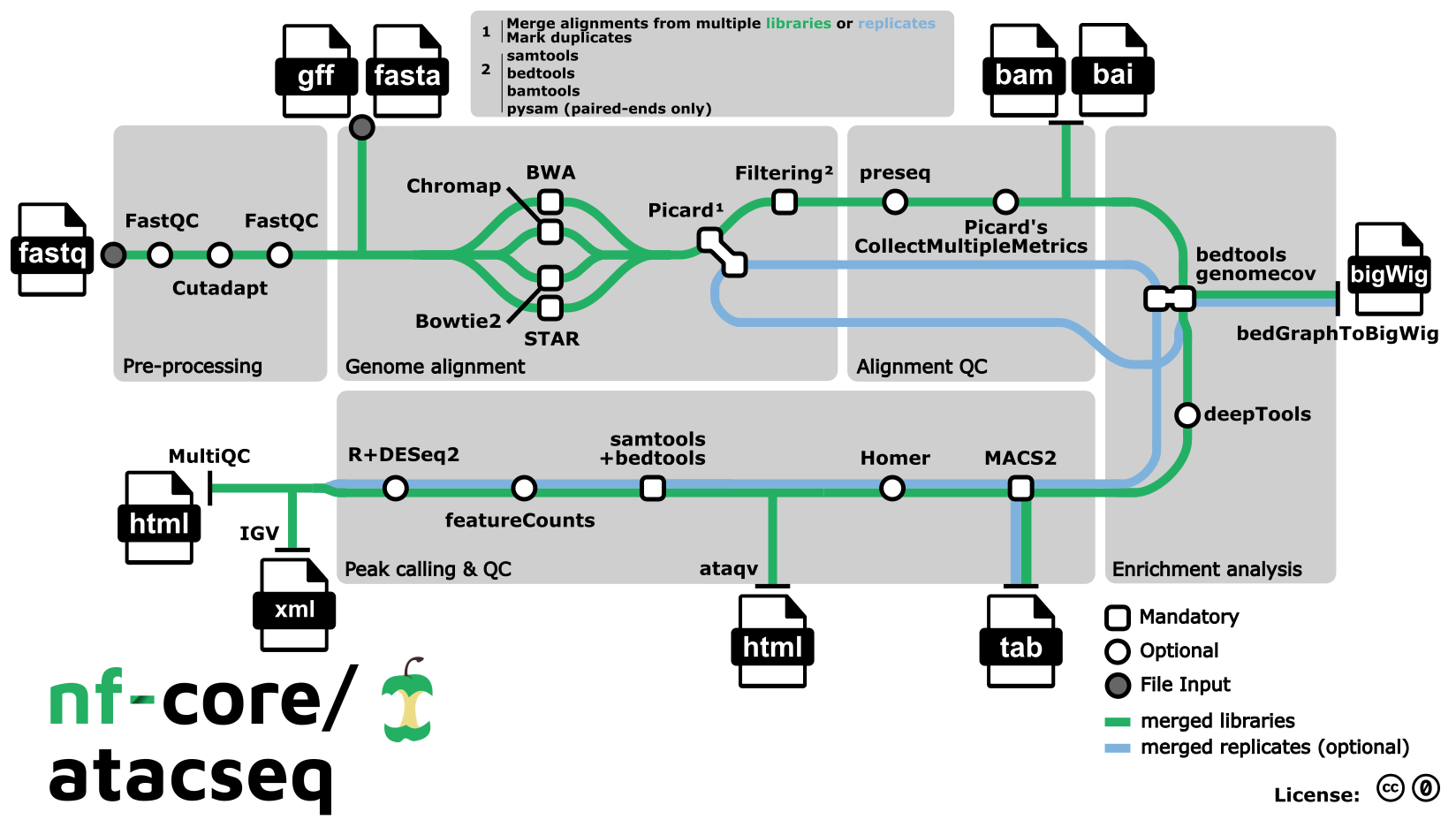
Figure 1. nf-core/atacseq workflow overview (version 2.1.2). Source: nf-core/atacseq.[1]
4.1 Read Processing and Alignment
FastQC assesses the raw FASTQ files. Trim Galore! uses Cutadapt to remove adapters and trim low-quality bases, followed by another quality check. Alignment options include BWA (default), Bowtie2, STAR, and Chromap. In version 2.1.2, paired-end data aligned with Chromap do not proceed beyond alignment.[1,5]
Picard marks duplicates and merges sequencing runs belonging to the same biological replicate. Duplicates are marked again before filtering. SAMtools, BEDTools, BAMTools, and Pysam remove mitochondrial reads, reads overlapping blacklisted regions, duplicates, and unreliable alignments, and check paired-end read consistency. These steps reduce technical noise before peak calling.[1]
4.2 Analysis After Filtering
| Task | Main tools | Purpose |
|---|---|---|
| Alignment and library QC | Picard, Preseq | Assess alignment quality and library complexity; estimate the benefit of deeper sequencing |
| Signal tracks | BEDTools, bedGraphToBigWig | Generate bigWig tracks scaled to one million mapped reads |
| Signal enrichment | deepTools | Examine signal around transcription start sites, across gene bodies, and genome-wide |
| Peak calling and annotation | MACS2, HOMER | Identify enriched regions and annotate their genomic context and nearby genes |
| Consensus regions and counting | BEDTools, featureCounts | Combine peaks into shared regions and count reads in each sample |
| Sample comparison and reporting | R/DESeq2, ataqv, MultiQC, IGV | Normalize counts, generate PCA and clustering plots, summarize QC, and visualize tracks |
These tasks correspond to the alignment QC, enrichment, peak calling, and reporting branches in the official diagram.[1,5]
4.3 Three Details to Keep in Mind
Library merging and biological replicate merging serve different purposes. Repeated sequencing runs of the same biological replicate use identical sample and replicate values in the samplesheet and are merged after alignment. Biological replicates within a condition share the same sample value but have different replicate values. The blue branch pools these replicates to increase coverage for peak calling. Read counting against the resulting consensus peaks still uses the separate replicate alignments, preserving differences between replicates.[5] See the samplesheet documentation for details.
Peak calling and consensus filtering have specific defaults. MACS2 calls broad peaks by default; --narrow_peak selects narrow peaks. The default consensus set is the union of peaks across samples, so a peak need not occur in every sample. Increasing --min_reps_consensus requires greater replicate support.[5]
PCA and clustering show how similar the samples are. The pipeline uses DESeq2 to generate these plots. Identifying significantly different accessibility between treatment and control requires a statistical comparison based on the experimental groups.[5]
5. What Does nf-core/atacseq Produce?
The experiment tags accessible DNA; the pipeline analyzes where those tags occur.
Version 2.1.2 organizes read QC, adapter trimming, alignment, filtering, peak calling, and reporting into a Nextflow workflow, with containers managing software dependencies.[1]
A peak is a genomic interval with significant enrichment of sequencing signal.
Three questions provide a useful starting point for reading the results:[5]
| Question | Relevant outputs |
|---|---|
| Is the data quality sufficient for further analysis? | MultiQC, ataqv, and associated QC metrics |
| Where are the accessibility signals? | MACS2 peaks and bigWig tracks |
| Can samples be compared across the same regions? | Consensus peaks, read count matrices, PCA, and clustering |
Consensus peaks combine the individual peak sets into shared genomic intervals for comparison.[5]
6. What Comes After Finding Accessible Regions?
ATAC-seq adds another perspective to genome analysis: how cells make DNA accessible and organize it into chromatin.
nf-core/atacseq provides a reusable workflow for analyzing these signals. The next step is to connect accessible regions with gene expression and experimental conditions, developing biological explanations that can be tested.