The Stupidest Machine Learning Mistakes in Bioinformatics
Your model has an AUROC of 0.98. The heatmap looks beautiful. The top genes have plausible biological functions.
Then you try another cohort. The performance falls apart.
Before replacing logistic regression with a transformer, inspect the experiment around the model. A sophisticated algorithm can learn a very simple mistake.
This post takes inspiration from the practical mistake-and-correction format of Chatomics’ bioinformatics mistakes article. The examples below are original teaching scenarios, not claims about experiments I have performed. “Stupid” describes a preventable workflow mistake, not the person making it.
1. Selecting genes before cross-validation
What you meant to do: Find a compact expression signature that predicts disease in new patients.
What you actually did: Use every patient’s disease label to select differentially expressed genes, then cross-validate a classifier on that fixed gene list.
The held-out patients have already helped choose the inputs. Cross-validation of the final classifier does not undo that information leak. This issue was documented in microarray classification more than two decades ago by Ambroise and McLachlan (2002).
Correction: Repeat supervised gene selection within each training fold. A gene list fixed independently of this dataset is a different situation; record where it came from.
# WRONG: validation labels influence the selected genes.
X_selected = SelectKBest(f_classif, k=100).fit_transform(X, y)
cross_val_score(classifier, X_selected, y, cv=cv, groups=patient_id)

# BETTER: the selector is fitted separately inside each fold.
model = make_pipeline(
    SelectKBest(f_classif, k=100),
    StandardScaler(),
    LogisticRegression(max_iter=2000),
)
cross_val_score(model, X, y, cv=cv, groups=patient_id)
These are workflow excerpts; imports and an explicit grouped splitter appear below. A pipeline protects the operations inside it. It cannot repair a leaked gene list prepared outside it.
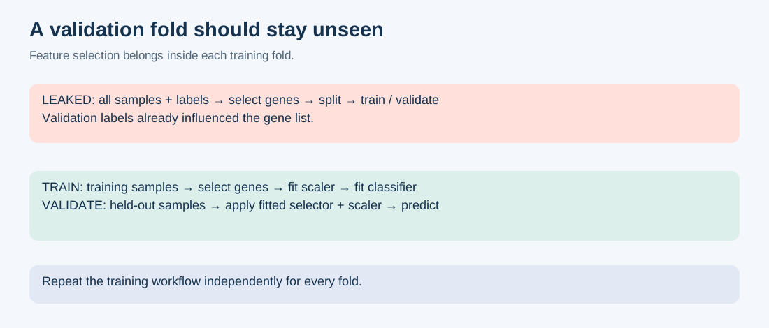
Figure 1. Original schematic. The top workflow lets validation labels influence gene selection. In the bottom workflow, each fold learns its own selector and scaler from training data only. No performance values are implied.
2. Splitting rows when you should split patients
What you meant to do: Predict an outcome for a patient the model has never seen.
What you actually did: Randomly split cells, pathology tiles, or repeated visits. Different observations from the same patient appear on both sides.
The model may exploit patient-specific expression, staining, or acquisition characteristics. A row-level score now answers a different question: can it predict more observations from partly familiar patients?
Correction: Keep the relevant independent unit together. For new-patient prediction, group by patient; for new-center deployment, also test a held-out center. For protein prediction, consider whether homologous sequences crossing the split undermine the intended claim.
Scikit-learn’s cross-validation guide explains grouped and time-ordered splitting. Stratifying labels does not itself separate patients.
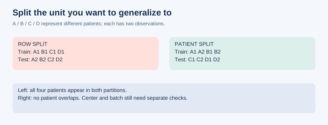
Figure 2. Original schematic. Letters A–D represent patients. Keeping all observations from one patient in the same partition prevents direct patient overlap; it does not guarantee freedom from center or batch confounding.
3. Learning preprocessing from the entire cohort
What you meant to do: Make features comparable before training.
What you actually did: Fit imputation, scaling, PCA, or data-driven batch adjustment on the whole cohort, then evaluate held-out samples.
Even without disease labels, a fitted transformation can use information about the evaluation distribution. For ordinary prediction of unseen samples, training data should determine the transformation. The official pitfalls guide explicitly includes scaling, imputation, PCA, and feature selection in its leakage discussion.
Correction: Fit learned transformations inside training folds; apply the fitted transformation to validation samples. Distinguish this from sample-local transformations, such as a fixed log transform, that do not estimate parameters from other samples.
Jointly integrating training and test cohorts can be appropriate for an explicitly transductive task, but it does not establish performance on future samples unavailable during fitting. Ask how a genuinely new sample would pass through the saved workflow.
4. Applying SMOTE before splitting
What you meant to do: Help the model learn a rare positive class.
What you actually did: Resample the complete dataset before cross-validation. Synthetic examples can depend on observations later assigned to validation, and evaluation no longer reflects the original class distribution.
Correction: Resample only the training portion of each fold. Keep validation and test observations untouched. An imblearn.pipeline.Pipeline handles samplers during fitting; the imbalanced-learn pitfalls guide demonstrates why resampling the whole dataset is problematic.
For a small, high-dimensional omics cohort, SMOTE is not automatically a good idea. A synthetic point between patients need not represent a biologically plausible patient. Compare against class weighting and a simple baseline before adopting it.
5. Tuning until the test set agrees with you
What you meant to do: Obtain an honest final performance estimate.
What you actually did: Try 30 gene panels, five algorithms, and several seeds; inspect the test score after each change; publish the winner.
The test set has become a model-selection tool. Cawley and Talbot (2010) explain how selection can overfit a noisy evaluation criterion, even when individual models are regularized.
Correction: Use development folds for tuning and keep a final test cohort untouched until the workflow is frozen. With limited samples, use nested cross-validation: the inner loop selects the model; the outer loop estimates the performance of that selection procedure. See the official nested-CV example.
Choosing the best random seed is also selection. Predeclare seeds or report the distribution across a planned set. The largest score is not a reproducibility strategy.
6. Celebrating 99% accuracy while finding zero positives
What you meant to do: Detect a rare outcome.
What you actually did: Report accuracy without examining the confusion matrix.
Consider 1,000 samples with 10 positives. A model that predicts “negative” for everyone has 99% accuracy and 0% recall. This is arithmetic, not a simulated benchmark.
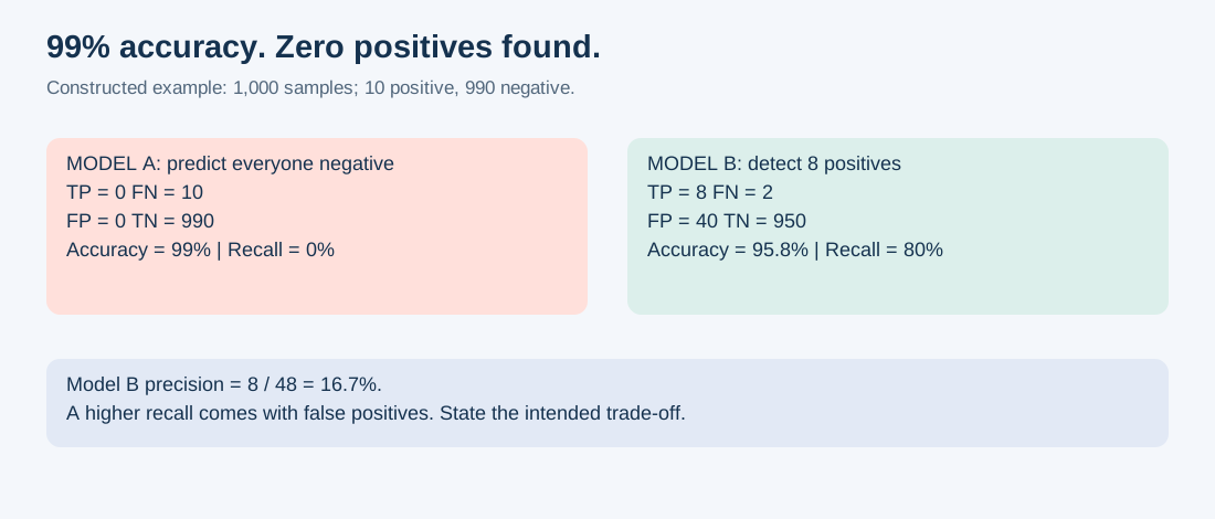
Figure 3. Constructed example, not patient data. Model A predicts everyone negative. Model B finds eight of ten positives but produces 40 false positives. B has lower accuracy; whether its trade-off is acceptable depends on the intended use.
Correction: State prevalence, show confusion counts, and report metrics suited to the task. Precision-recall summaries can be informative when positives are rare; their baseline and interpretation depend on prevalence. AUROC measures ranking, not performance at a chosen operating threshold. The metric guide defines these quantities.
Also compare with a DummyClassifier. Beating no baseline is an easy way to impress yourself.
7. Treating 0.5 as a scientific threshold
What you meant to do: Turn a risk score into an actionable decision.
What you actually did: Accept the library’s default cutoff and interpret a score of 0.9 as a trustworthy 90% probability.
Ranking, calibration, and decision-making are separate properties. A model can rank samples well while producing poor probability estimates. Inspect a reliability diagram; the calibration guide explains this distinction. Brier score is useful, but it reflects more than calibration alone.
Correction: Select a threshold using a stated objective and development data, then evaluate that fixed threshold on held-out data. Do not optimize it on the final test set. The threshold guide shows why changing the cutoff changes decisions without changing the underlying probability scores.
Calibration also needs separation from model fitting and final evaluation. Recheck it when cohort composition or prevalence changes.
8. Training a batch detector and calling it a disease model
What you meant to do: Learn biology associated with disease.
What you actually did: Collect all cases in one laboratory and all controls in another, then randomly split the combined dataset.
Both partitions preserve the same technical shortcut. A high test score may reflect the laboratory, processing date, or assay rather than disease.
This is more than a hypothetical concern: Zech et al. (2018) found that pneumonia models could exploit hospital information and did not consistently generalize across sites. Applying that lesson to omics is an analogy, not a result reported in that imaging paper.
Correction: Audit outcome-by-batch tables, compare metadata-only baselines, and evaluate relevant external cohorts. If batch and disease are perfectly confounded, a batch-correction button cannot establish which signal was biological. You need a design that separates them.
Likewise, a prognosis model must use information available at the stated prediction time. Post-outcome measurements can make an impossible prediction look easy.
9. Turning feature importance into a mechanism
What you meant to do: Understand why the model predicts well.
What you actually did: Label the highest-ranked gene a disease driver.
Feature importance describes a model’s behavior under an explanation procedure. It does not by itself identify a causal biological mechanism. Coexpressed genes also complicate interpretation: if one gene substitutes for another, permuting either alone may have little effect.
Correction: Assess importance on held-out data, inspect correlated feature groups, and check stability across folds or cohorts. The permutation-importance guide and its correlated-feature example explain why a useful predictor can still receive low permutation importance.
Use an important gene as a candidate for follow-up, and state the additional evidence needed for a mechanistic claim.
10. Losing sample identity in a perfectly valid array
What you meant to do: Match each expression profile to its label.
What you actually did: Sort the expression table, leave metadata in its original order, convert both to NumPy, and start training.
Everything has the right shape. Nothing has the right patient.
Correction: Join by explicit identifiers, reject duplicates, and assert order before dropping labels. Keep feature names and their order with the fitted model too.
# X_df: samples × genes; metadata: one row per sample_id.
assert X_df.index.is_unique
assert metadata["sample_id"].is_unique
meta = metadata.set_index("sample_id").loc[X_df.index]
assert X_df.index.equals(meta.index)
assert meta["outcome"].notna().all()
y = meta["outcome"].to_numpy()
For longitudinal data, use a unique observation ID for alignment and a separate patient ID for splitting. Do not force multiple visits into a one-row-per-patient assumption.
A small workflow worth keeping
The following is a template for binary classification with patient groups, not a complete omics pipeline or a benchmark. X must already be correctly aligned, numeric, and free of missing values; y is binary and patient_id identifies groups. Ensure sufficient class representation and groups in every fold. Set k to suit the available features.
import numpy as np
from sklearn.feature_selection import SelectKBest, f_classif
from sklearn.linear_model import LogisticRegression
from sklearn.model_selection import StratifiedGroupKFold, cross_validate
from sklearn.pipeline import make_pipeline
from sklearn.preprocessing import StandardScaler

cv = StratifiedGroupKFold(n_splits=5, shuffle=True, random_state=42)
for train, valid in cv.split(X, y, groups=patient_id):
    assert not (set(patient_id[train]) & set(patient_id[valid]))
    assert len(np.unique(y[train])) == len(np.unique(y[valid])) == 2

model = make_pipeline(
    SelectKBest(f_classif, k=100),
    StandardScaler(),
    LogisticRegression(max_iter=2000),
)
scores = cross_validate(
    model, X, y, groups=patient_id, cv=cv,
    scoring={"auroc": "roc_auc", "ap": "average_precision"},
)
print(scores["test_auroc"])
print(scores["test_ap"])
This evaluates a fixed workflow. If you use these scores to choose k, regularization, or algorithms, add an inner selection loop and retain an outer evaluation loop. Five correlated fold scores are not five independent experiments or automatically a confidence interval. These snippets were checked for syntax, not run against a biological dataset.
Before believing the next impressive score
Ask four questions: Who is held out? What information crossed the boundary? Which decision does the metric support? Can a simpler explanation account for the result?
Save the split IDs, feature schema, preprocessing objects, environment versions, and selection history. A fixed seed helps replay a workflow; it does not make the workflow valid.
The most expensive mistake is often the one that produces a beautiful figure and no error message.
Sources checked October 12, 2026. Linked documentation is version-dependent; pin the versions used in a real analysis. All three figures are original educational illustrations.